import gzip
from pathlib import Path
from ase.build import molecule
import matplotlib.pyplot as plt

from chemparseplot.parse.orca import geomscan

---------------------------------------------------------------------------
ModuleNotFoundError                       Traceback (most recent call last)
Cell In[1], line 3
      1 import gzip
      2 from pathlib import Path
----> 3 from ase.build import molecule
      4 import matplotlib.pyplot as plt
      6 from chemparseplot.parse.orca import geomscan

ModuleNotFoundError: No module named 'ase'

Geometry Scan#

Often it is of interest to scan for energies over a particular aspect of molecular geometry. Here we consider the example of scanning over the bond length of the H2 molecule.

System construction#

For simplicity, we will just use ase for this:

h2 = molecule("H2")
h2.write("data/h2_base.xyz", comment="\n")

This can be visualized via ase gui h2_base.xyz or similar, to see[1]:

H2 Molecule

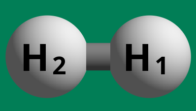
Note that for ORCA, we need the “plain” .xyz file, so we need to remove the metadata added by ase, hence the newline comment.

ORCA Input#

To run orca, we can use an input file such as:

!OPT UHF def2-SVP
%geom Scan
 # B <atmid1> <atmid2> = init, final, npoints
 # Converted from Angstrom to Bohr
 B 0 1 = 7.5589039543, 0.2116708996, 33
 end
end
*xyzfile 0 1 h2_base.xyz

Execution#

Following the best practices for running ORCA, we have[2]:

export PATH=$PATH:/blah/orca_5_0_4_linux_x86-64_openmpi411/
mkdir uhf
cp orca.inp h2_base.xyz uhf
cd uhf
($(which orca) orca.inp 2>&1) | tee scan_uhf

Also because it is annoying to keep blobs of text, and because it is large:

gzip -9 -c scan_uhf > scanuhf.gz
mv scanuhf.gz ../data/

Analysis with `chemparseplot`#

Now we can finally get to the good bit. Rather than painstakingly parsing “by eye” the scan_uhf file, we will simply use chemparseplot:

orcaout = gzip.open(Path("data/scanuhf.gz"), 'rt').read()
act_energy = geomscan.extract_energy_data(orcaout, "Actual")
print(act_energy)

Note that there are units attached, which makes subsequent analysis much easier, since pint will ensure that the correct units are always used.

act_energy[0].to('angstrom')

Plotting#

This is simple enough to plot.

fig, ax = plt.subplots(figsize=(4, 4), dpi=100)
ax.scatter(act_energy[0].magnitude, act_energy[1].magnitude)

However, this is not super satisfying, and since this is a “supported” workflow, we can leverage chemparseplot instead.

# Create an instance of TwoDimPlot
twodim_plot = TwoDimPlot()

# Set the units for the plot
twodim_plot.set_units('angstrom', 'hartree')

# Add data (EnergyPath instances) to the plot
energy_path1 = EnergyPath('Path 1', np.linspace(0, 10, 30) * ureg.angstrom, np.random.uniform(-1, 0, 30) * ureg.hartree)
energy_path2 = EnergyPath('Path 2', np.linspace(1, 9, 25) * ureg.angstrom, np.random.uniform(-0.5, 0.5, 25) * ureg.hartree)
twodim_plot.add_data(energy_path1)
twodim_plot.add_data(energy_path2)

# Display the plot
twodim_plot.show_plot("Energy Paths")

twodim_plot.set_units('bohr', 'electron_volt')

twodim_plot.fig